Abstract
When an earthquake happens, how are scientists able to determine the original location of the quake? In this project, you'll use archived data from a network of seismometers to find out for yourself. You'll create your own seismograms from the comfort of your own computer with an easy-to-use webpage interface. Then you'll analyze your seismograms to determine the distance of the quake from each seismometer station. By mapping your analyzed data, you will be able to determine the location of the quake.Summary
Sources
- Thanks to Dr. Peggy Hellweg, Berkeley Seismology Laboratory (BSL), for suggesting this project, which is based on a laboratory exercise she wrote.
- The seismograms in this project were generated using the 'Make Your Own Seismogram!' webpage: UC Regents, 2005a. Make Your Own Seismogram! Northern California Earthquake Data Center, University of California, Berkeley and USGS. Retrieved December 21, 2006.

Objective
The goal of this project is to locate the epicenters of Northern California earthquakes using archived seismometer data.Introduction
A fundamental principle of geology is that the features of the Earth are not fixed. Instead, they change over time. The time scale of most geologic changes is creepingly slow in terms of a human lifetime. Uplift of mountain ranges may occur at 1-10 mm/year, not even a hill in a human lifetime, but when continued over millions of years it results in some spectacular peaks!
An earthquake is an example of a major geologic event that occurs suddenly. If you look at a map of historic earthquakes (USGS, 2007), you'll notice that most quakes occur near the boundaries between tectonic plates. At boundaries where the plates oppose one another, tremendous strains can build up between between the plates. The strains are suddenly released when one plate slips against the other. The energy from this sudden movement travels through the earth as shock waves.
Figure 1 is from a US Geological Survey publication, "The Interior of the Earth" (Robertson, date unknown). It shows the layers of the Earth, through which the shock waves travel.
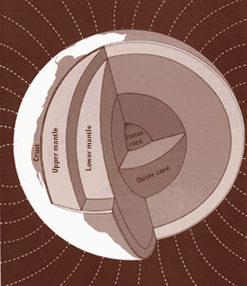
Figure 1. The layers of the Earth (Robertson, date unknown).
Table 1, from the same publication, gives a brief description of each of the earth's layers (Robertson, date unknown).
| Layer | Thickness (km) |
Density (g/cm3) | Types of Rock Found | |
| Top | Bottom | |||
| Crust | 30 | 2.2 | 2.9 | Silicic rocks. Andesite, basalt at base. |
| Upper mantle | 720 | 3.4 | 4.4 | Peridotite, eclogite, olivine, spinel, garnet, pyroxene. Perovskite, oxides at bottom. |
| Lower mantle | 2,171 | 4.4 | 5.6 | Magnesium and silicon oxides. |
| Outer core | 2,259 | 9.9 | 12.2 | Iron+oxygen, sulfur, nickel alloy. |
| Inner core | 1,221 | 12.8 | 13.1 | Iron+oxygen, sulfur, nickel alloy. |
The shock waves spreading out from an earthquake are called seismic waves (from the Greek word for earthquake). There are two general types of seismic waves: body waves and surface waves.
- Body waves travel through the Earth's interior.
- Surface waves, which are analogous to water waves, travel just beneath the Earth's surface.
There are two types of body waves, P waves and S waves. P waves (also called primary waves) are compression waves. Like sound waves, they consist of compressions and rarefactions of the material through which they travel. The compressions and rarefactions are in the same direction that the wave is traveling. S waves (also called secondary waves) are transverse (or shear) waves, meaning that the ground moves perpendicularly to the direction of travel. S waves have much higher amplitude than P waves, but travel more slowly. They carry more destructive force than P waves. Another difference between P waves and S waves is that S waves cannot travel through the Earth's liquid core, while P waves can. S waves can therefore be detected by seismometers near the epicenter of an earthquake, but not by more distant seismometers. P waves can be detected by both local and distant seismometers.
Figure 2 (Robertson, date unknown) is a cross-section of the Earth, showing how P waves and S waves travel through the various layers. Because of the varying density of the layers, the waves are refracted as they pass through the different layers. This is analogous to the refraction of light waves when they pass from air to water, for example.
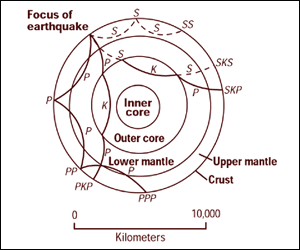
A diagram of a cross-section of the Earth shows how earthquake waves travel in curved lines through the inner layers of the Earth. Waves are able to travel through the crust, upper mantle, lower mantle, and outer core but are unable to travel through the inner core.
Figure 2. "Cross section of the whole Earth, showing the complexity of paths of earthquake waves. The paths curve because the different rock types found at different depths change the speed at which the waves travel. Solid lines marked P are compressional waves; dashed lines marked S are shear waves. S waves do not travel through the core but may be converted to compressional waves (marked K) on entering the core (PKP, SKS). Waves may be reflected at the surface (PP, PPP, SS)." (Robertson, date unknown).
Figure 3 is a seismometer trace that shows P waves and S waves from a local earthquake. Since P waves travel faster than S waves, they always arrive first. The S wave is marked by an abrupt increase in the amplitude of the disturbance on the trace. In this project you will use a webpage interface to make similar seismograms in order to locate earthquake epicenters.
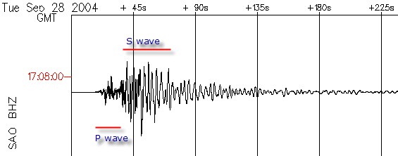
An example seismogram dated Sep. 28, 2004, and labeled SAO BHZ, shows that P-waves are the first signs that an earthquake is occuring. S-waves generated by an earthquake follow the P-waves. When compared the P-waves have a smaller amplitude and higher frequency than the S-waves.
Figure 3. Example seismogram created with the 'Make Your Own Seismogram!' webpage (UC Regents, 2005a).
The difference in travel time between the first P wave and the first S wave can be used to measure the distance from the seismometer recording station to the epicenter of a local earthquake. In this project you will use this method to determine the location of earthquakes using archived data from the Berkeley Digital Seismic Network.
Terms and Concepts
To do this project, you should do research that enables you to understand the following terms and concepts:- Plate tectonics
- Earthquake
- Temblor
- Epicenter
- Seismometer
- Coordinated Universal Time (UTC)
- Seismic waves:
- Body waves, including P-waves and S-waves (also called P and S phases)
- Surface waves
- Earth layers:
- Crust
- Upper mantle
- Lower mantle
- Outer core
- Inner core
- Travel time
Questions
- Can you explain the differences between P-waves and S-waves?
- What causes earthquakes?
- Where do earthquakes occur most frequently?
Bibliography
To help you get started on you background research, here are some useful websites on the passage of seismic waves through Earth's interior and a good general introduction to waves:- Robertson, E.C. (2011, January 14). The Interior of the Earth. United States Geological Survey (USGS). General Interest Report. Retrieved March 8, 2013.
- Louie, J. (1996, Oct. 10). Earth's Interior. The Nevada Seismological Laboratory, University of Nevada. Retrieved March 8, 2013.
- Henderson, T. (n.d.). Waves. The Physics Classroom. Retrieved March 8, 2013.
- The Regents of the University of California. (2012, Apr. 25). Make Your Own Seismogram! Northern California Earthquake Data Center, University of California, Berkeley, and USGS. Retrieved March 8, 2013.
- The Regents of the University of California. (n.d.). Map of BDSN sites. Berkeley Seismological Lab, University of California, Berkeley. Retrieved March 8, 2013.
- USGS. (n.d.). Search Earthquake Catalog. U.S. Department of the Interior. Retrieved April 9, 2018.
- California Integrated Seismic Network (CISN). (2004, Sept. 28). 2004 Parkfield Earthquake: Comparison with the Forecast. Northern California Management Center, USGS, Berkeley Seismological Laboratory. Retrieved March 8, 2013.
Materials and Equipment
To do this experiment you will need the following materials and equipment:- Computer with Internet access and printer
- Metric ruler
- Pencil
- Compass
- A helper
Experimental Procedure
Introduction: A Brief Summary of the Method
- In principle, the method for locating the epicenter of an earthquake is fairly simple. Here are the steps:
- Create your seismogram.
- Identify the beginning of the P-wave and the S-wave on the seismogram, and determine the time of each of these events.
- Calculate the time difference between the arrival of the S-wave and the arrival of the P-wave.
- Use the Travel Time graph (available below) to find the distance from the station to the event and the Origin Time.
- Using the distance scale on the station map, set your compass to the correct distance and draw a circle on the map, centered on the station.
- Repeat this process for at least two more stations.
- The epicenter will be located in the region where the circles overlap.
- In practice, there are some difficulties with this method.
- For some stations, you may find it difficult (or even impossible) to identify the beginning of the S-wave with precision. In this case, you can use the origin time and the arrival of the P-wave at the station to calculate the distance.
- Sometimes, you may have to go back and study the seismogram again. For example, you may have two or more 'hunches' about the precise location of the arrival of the S-wave. You try one of your hunches, and later find that your circles do not overlap well. Go back and try your second hunch, and see if the overlap is improved.
- You may also want to try adjusting the parameters used for creating the seismogram.
- We'll discuss these difficulties as we work through an example.
Working Through an Example: The Parkfield Quake of 2004
- Make a list of Northern California earthquakes. Have a helper visit the USGS website, https://earthquake.usgs.gov/earthquakes/search/, and make a list of at least three Northern California earthquakes (of magnitude 3.5 or greater).
- Have your helper write down the date and approximate time of the quake (round down to the nearest 5 minutes).
- On a separate piece of paper, they should write down the following information for each quake:
Date
(yyyy/mm/dd)Time
(hh:mm:ss, UTC)Location Coordinates
(latitude and longitude)Magnitude
- When you have completed your analysis for the location of each of the quakes, open the envelope and see how accurate you were!
- For each quake on the list that your helper gives you, make seismograms from at least three different stations. The webpage for making a seismogram (UC Regents, 2005a) is pretty straightforward. We'll walk through an example to show you how to use it. In this example, our helper gave us the date September 28, 2004, and the time 17:15:00 UTC.
- Select a station. Click on one of the radio buttons to select from the 28 available stations (see illustration, below). For a map of the station locations, see UC Regents, 2005b. Here is a Map of BDSN sites. For our example seismogram, we used data from station SAO, at the San Andreas Geophysical Observatory in Hollister, CA.
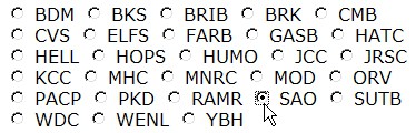
A cropped screenshot from the website earthquake.usgs.gov shows 28 different stations with radio buttons that are selectable when setting parameters for generating a seismogram on the website earthquake.usgs.gov. The station labeled SAO was selected to generate an example graph.
- Select the data channel. There are two types of data channels: 'long period' and 'broadband.' The broadband channels are good for analyzing local earthquakes, so you should use these channels for this project. You can choose to look at vertical motion, or horizontal motion (either north-south or east-west). We chose to look at the vertical channel (BHZ) for our seismograms.
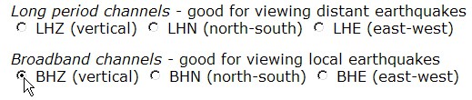
A cropped screenshot from the website earthquake.usgs.gov shows 6 different channels that are selectable when setting parameters for generating a seismogram. There are three long period channels (LHZ[vertical], LHN[north-south], LHE9east-west]) and three broadband channels (BHZ[vertical], BHN[north-couth], BHE[east-west]). The broadband channel BHZ was selected for the example graph.
The broadband channels collect information more frequently than the long-period channels, and so have information about higher-frequency waves. Long-period channels are good for viewing seismic activity from distant earthquakes. See the Variations section for project ideas that can make use of the long-period data channels. - Set the desired time period. The seismogram plot can be a maximum of 1 hour for broadband data channels (24 hours for long-period data channels). As you'll see in step 3c, we played around with the time parameters so that our example seismogram displayed only a single trace. We used a compression factor of 10 (more on this in the next step), which means that each trace will be 7 and a half minutes in duration. Enter the date and time in the format "yyyy/mm/dd,hh:mm:ss". Separate date and time with a comma, but no spaces. Remember that the time is given in Coordinated Universal Time (UTC), not local time. In the screenshot, we have set the plot to cover a 37.5 minute stretch on September 28, 2004, both before and after the time our helper gave us (17:15:00, UTC).
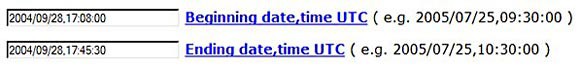
A cropped screenshot from the website earthquake.usgs.gov shows beginning and ending dates and times that can be set as parameters when creating a seismogram. Time must be given in Coordinated Universal Time and in the format yyyy/mm/dd,hh:mm:ss.
You may notice that the trace starts somewhere in the middle of the graph. The graphing program automatically sets the starting times for each trace, based on the compression factor used. - Set the plotting parameters. You will probably need to adjust the plotting parameters in order to get good-looking traces. Here is a brief description of what each parameter does (there is also a help page available: How To Make Your Own Seismogram!). If in doubt, just try adjusting one parameter at a time to see what changes! You can always hit the 'Back' button on your browser to make a change and try again.
- The 'Compression factor' controls the x-axis scaling of the seismogram.
- The 'Amplitude scaling' controls the y-axis scaling of the seismogram. This parameter may need adjustment for each station. You'll have an easier time comparing the traces from different stations if you try to make them roughly similar in amplitude.
- The 'Pixels between adjacent output traces' controls the spacing between successive traces (if your plot requires more than one trace).
Here are the parameters we used for the SAO seismogram:

A cropped screenshot of the website earthquake.usgs.gov shows three factors compression factor, amplitude scaling and pixels between adjacent output traces that can be adjusted when generating a seismogram. Each factor controls a different aspect of the seismogram: x-axis scaling, y-axis scaling and space between traces respectively. In this example the compression factor is set to 10, the amplitude scaling to .0000125, and the pixels between adjacent output traces to 20.
- Make the seismogram! Click on the "Create Plot" button near the bottom of the page. That's it! Here's the resulting seismogram:
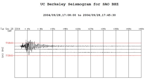
With a compression factor of ten, each trace lasts 450 seconds (7.5 minutes). The UTC time is labeled every fourth trace (red traces). To show this earthquake as a single trace, you could set the start time to 17:15:30, and the end time to 17:23:00 (as we did for the seismogram displayed in step 3c, below). Unfortunately, you can't control when the traces start; the graphing algorithm determines that automatically. Changing the compression factor will sometimes change the trace start time.
- Select a station. Click on one of the radio buttons to select from the 28 available stations (see illustration, below). For a map of the station locations, see UC Regents, 2005b. Here is a Map of BDSN sites. For our example seismogram, we used data from station SAO, at the San Andreas Geophysical Observatory in Hollister, CA.
- Analyze the seismogram.
- Identify the a'rival of the P-wave. The P-wave always arrives first. Use a ruler and the seismogram scale to calculate a precise time. For example, if the distance you measure between 0 and +45 s is 2.30 cm, and the distance you measure from 0 to the start of the P-wave is 0.85 cm, then the elapsed time is: (0.85/2.30) x 45 s = 16.6 seconds. Add this elapsed time to the time at the start of the trace (17:15:30) to get the P-wave arrival time.
- Identify the arrival of the S-wave. Again, use a ruler and the seismogram scale to calculate a precise time. Remember that the S-wave may be difficult to identify, because the trace is already disturbed by the P-wave and other waves associated with it.
- Here is a detail view of the SAO station trace. The P-waves and S-waves are indicated. Note that it is difficult to determine the precise arrival time of the S-wave, since the trace is already disturbed by the P-wave.
An example seismogram dated Sep. 28, 2004, and labeled SAO BHZ, shows that P-waves are the first signs that an earthquake is occuring. S-waves generated by an earthquake follow the P-waves. When compared the P-waves have a smaller amplitude and higher frequency than the S-waves.
- Figure out the time of arrival of each wave and enter it in a data table in your lab notebook like the one below:
Station P-wave arrival time
(Tp, hh:mm:ss)S-wave arrival time
(Ts, hh:mm:ss)Ts − Tp
(s)Tp − T0
(s)
(optional)Distance
(km)Origin Time (T0)
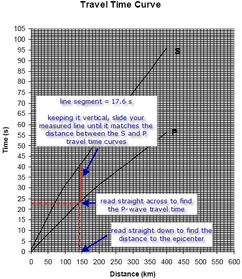
(hh:mm:ss)SAO P 17:15:47 (S) 17:16:04.6 17.6 − 142 23
- If you are uncertain about your identification of the S-wave, put parentheses around it when you enter it in the table, like this: (S) 17:15:49. That way, if you have to repeat some measurements later, you'll be able to identify which ones to re-examine.
- Calculate the difference in arrival times of the first S-wave and the first P-wave. (If you have not identified an S-wave arrival, do not calculate this time.) Remember that there are 60 seconds in one minute and 60 minutes in one hour. Enter the information in the data table.
- Use the Travel Time Graph (below) to find the distance from the station to the event.
- For a printable copy of the Travel Time Graph (requires Adobe Acrobat Reader).
- Use the y-axis of the travel time graph to make a vertical scale on the edge of a piece of paper.
- Mark the elapsed time between the P-wave arrival and the S-wave arrival.
- Slide the scale along the travel time curve until the distance you marked matches the space between the S and P travel time curves. Keep your scale parallel to the vertical axis as you do this.
- Read the distance at this point from the x-axis.
- Enter the distance in your data table.
- From the P-wave curve at this point, read across to the travel time. By subtracting this time from the arrival time of the P-wave, you can get an estimate for the time of the earthquake at the origin. Enter the Origin Time in your data table.
- This figure illustrates the whole process for determining the distance to station SAO.
A cropped screenshot of the website earthquake.usgs.gov shows 28 different stations with radio buttons that are selectable when setting parameters for generating a seismogram on the website earthquake.usgs.gov. The station labeled SAO was selected to generate an example graph.
- Draw a circle on the station map to indicate the possible locations for the earthquake epicenter.
- Use the map scale to set your compass to the correct distance (as determined from the travel time graph). Since the map scale is only 100 km, you will probably need to use your ruler to measure and extend the scale.
- With your compass set correctly, place the point of the compass on the station, and draw a circle around it. The origin of the earthquake should lie on (or near) this circle.
- Here is a map for locating the epicenter of the Parkfield quake, with circles marked for stations SAO, KCC, and CMB. Which station would you examine next for additional information?
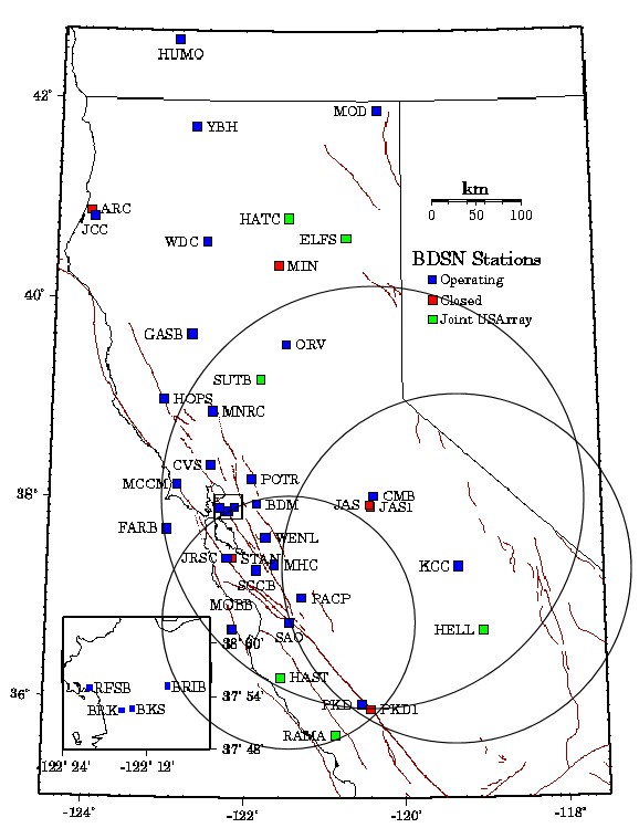
A map of the coast of Northern California shows seismometer stations represented by blue, red and green squares. Each square has sequence of 3 or 4 letters next to it to identify each station. Blue squares are stations that are in operation, red squares are closed stations and green squares are stations that are joint with the USArray. Three circles are drawn around three stations and overlap which represents the distance an earthquake should have occured from each of the three stations. The smallest circle is drawn around the SAO station, the second largest circle is drawn around the KCC station and the largest circle is drawn around the CMB station.
- Add more stations to pinpoint the epicenter location. Repeat steps 2-4 for additional stations until you are confident about the location of the epicenter.
- When making additional seismograms, examine the data you have already plotted on the station map and think carefully about which station will provide the most valuable additional information.
- Remember that you may have to go back and reassess your determination of the S-wave arrival time on some seismograms.
- When you are confident of your results, mark your predicted epicenter location on the map.
- Repeat the process for all of the earthquakes on your list. When you are finished, open the envelope with the table of actual locations and times and find out how accurate your predictions were!
Ask an Expert
Global Connections
The United Nations Sustainable Development Goals (UNSDGs) are a blueprint to achieve a better and more sustainable future for all.

Variations
- How closely do your origin times calculated from the different seismometer stations agree? Can you estimate the amount of uncertainty in your predicted origin time? One idea for estimating the uncertainty would be to examine the traces carefully and try to put upper and lower bounds on the S-wave arrival time. You could then draw two circles for each station to indicate the upper and lower bounds on the distance estimate from the travel time graph.
- For a more basic project, see: the Science Buddies project How Fast Do Seismic Waves Travel?
- If you'd like to try your hand at building a seismograph, see the Science Buddies project Is There a Whole Lot of Shaking Going On? Make Your Own Seismograph and Find Out!
Careers
If you like this project, you might enjoy exploring these related careers:


Related Links
- Science Fair Project Guide
- Other Ideas Like This
- Geology Project Ideas
- Big Data Project Ideas
- My Favorites