Summarizing Your Data
Key Info
So now you have collected your raw data, and you have results from multiple trials of your experiment. How do you go from piles of raw data to summaries that can help you analyze your data and support your conclusions?
Fortunately, there are mathematical summaries of your data that can convey a lot of information with just a few numbers. These summaries are called descriptive statistics. The following discussion is a brief introduction to the two types of descriptive statistics that are generally most useful:
- summaries that calculate the "middle" or "average" of your data; these are called measures of central tendency, and
- summaries that indicate the "spread" of the raw measurements around the average, called measures of dispersion.
Mean, Median, and Mode
Measures of Central Tendency: Mean, Median, and Mode
In most cases, the first thing that you will want to know about a group of measurements is the "average." But what, exactly, is the "average?" Is it the mathematical average of our measurements? Is it a kind of half-way point in our data set? Is it the outcome that happened most frequently? Actually, any of these three measures could conceivably be used to convey the central tendency of the data. Most often, the mathematical average or mean of the data is used, but two other measures, the median and mode are also sometimes used.
We'll use a plant growth experiment as an example. Let's say that the experiment was to test whether plants grown in soil with compost added would grow faster than plants grown in the same soil without compost. Let's imagine that we used six separate pots for each condition, with one plant per pot. (In many cases, your project will have more than six trials. We are using fewer trials to keep the illustration simpler.) One of the growth measures chosen was the number of leaves on each plant. Suppose that the following results were obtained:
| Plant Growth Without Compost (# of leaves/plant) |
Plant Growth With Compost (# of leaves/plant) |
| 6 | 5 |
| 4 | 9 |
| 5 | 9 |
| 4 | 11 |
| 8 | 8 |
| 3 | 6 |
Mean
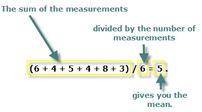
The mean value is what we typically call the "average." You calculate the mean by adding up all of the measurements in a group and then dividing by the number of measurements. For the "without compost" case, the mean is 5, as you can see in the illustration.
For the "with compost" case, the mean is 8. Use the numbers in the table mentioned to do the calculation for yourself to confirm that this is correct.
Median and Mode
The easiest way to find the median and the mode is to first sort each group of measurements in order, from the smallest to the largest. Here are the values sorted in order:
| Plant Growth Without Compost (# of leaves/plant) |
Plant Growth With Compost (# of leaves/plant) |
| 3 | 5 |
| 4 | 6 |
| 4 | 8 |
| 5 | 9 |
| 6 | 9 |
| 8 | 11 |
The median is a value at the midpoint of the group. More explicitly, exactly half of the values in the group are smaller than the median, and the other half of the values in the group are greater than the median. If there are an odd number of measurements, the median is simply equal to the middle value of the group, when the values are arranged in ascending order. If there are an even number of measurements (as here), the median is equal to the mean of the two middle values (again, when the values are arranged in ascending order). For the "without compost" group, the median is equal to the mean of the values of the 3rd and 4th values, which happen to be 4 and 5:
Notice that, by definition, three of the values (3, 4, and 4) are less than the median, and the other three values (5, 6, and 8) are greater than the median. What is the median of the "with compost" group
The mode is the value that appears most frequently in the group of measurements. For the "without compost" group, the mode is 4, because that value is repeated twice, while all of the other values are only represented once. What is the mode of the "with compost" group?
It is entirely possible for a group of data to have no mode at all, or for it to have more than one mode. If all values occur with the same frequency (for example, if all values occur only once), then the group has no mode. If more than one value occurs at the highest frequency, then each of those values is a mode. Here is an example of a group of raw data with two modes:
The two modes of this data set are 26 and 41, since each of those values appears twice, while all the other values appear only once. A data set with two modes is sometimes called "bimodal." Multimodal data sets are also possible.
Mean, Median, or Mode: Which Measure Should I Use?
What's the difference between these measures? When would you choose to use one in preference to another? The following illustration shows the mean, median, and mode of the "without compost" data sample on a graph. The x-axis shows the number of leaves per plant. The height of each bar (y-axis) shows the number of plants that had a certain number of leaves. (Compare the graph with the data in the table, and you will see that all of the raw data values are shown in the graph.) This graph shows why the mean, median, and mode are all called measures of central tendency. The data values are spread out across the horizontal axis of the graph, but the mean, median, and mode are all clustered towards the center. Each one is a slightly different measure of what happened "on average" in the experiment. The mode (4) shows which number of leaves per plant occurred most frequently. The median (4.5) shows the value that divides the data points in half; half of the values are lower and half of the values are higher than the median. The mean (5) is the arithmetic average of all the data points.
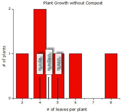
A histogram includes a marker to indicate the values of the mean, median and mode. The mode is 4 since it is the value that appears the most often. The median is 4.5 since the set of numbers is even, and the mean is 5 since the values of the numbers added together are evenly divisible by the number of values added.
In general, the mean is the descriptive statistic most often used to describe the central tendency of a group of measurements. Of the three measures, it is the most sensitive measurement, because its value always reflects the contributions of each of the data values in the group. The median and the mode are less sensitive to "outliers"—data values at the extremes of a group. Imagine that, for the "without compost" group, the plant with the greatest number of leaves had 11 leaves, not 8. Both the median and the mode would remain unchanged. (Check for yourself and confirm that this is true.) The mean, however, would now be 5.5 instead of 5.0.
On the other hand, sometimes it is an advantage to have a measure of central tendency that is less sensitive to changes in the extremes of the data. For example, if your data set contains a small number of outliers at one extreme, the median may be a better measure of the central tendency of the data than the mean.
If your results involve categories instead of continuous numbers, then the best measure of central tendency will probably be the most frequent outcome (the mode). For example, imagine that you conducted a survey on the most effective way to quit smoking. A reasonable measure of the central tendency of your results would be the method that works most frequently, as determined from your survey.
It is important to think about what you are trying to accomplish with descriptive statistics, not just use them blindly. If your data contains more than one mode, then summarizing them with a simple measure of central tendency such as the mean or median will obscure this fact. Table 1 is a quick guide to help you decide which measure of central tendency to use with your data.
| First, what are you trying to describe? | Second, what does your data look like? | Then, the best measure of central tendency is... |
| Groups, or classes of things. Survey results often fall in this category, such as, "What is the most effective way to quit smoking?" or "Gender Differences in After-School Activities" |
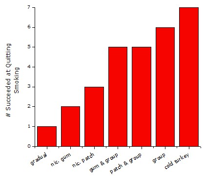 A hypothetical graph of survey responses shows that quitting cold-turkey was the most answered response to a survey on effective ways to stop smoking. |
Mode. In these made-up survey results, 'cold turkey' is the most frequent response. |
| Position on a ranking scale, such as: 1-5 stars for movies, books, or restaurants |
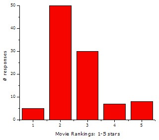 A hypothetical graph of movie review scores from 1 to 5 has numerical values serving as a ranking scale. A score of 2 was given the most by 50 participants, a score of 1 was given the least with only 5 participants. |
Median. The median movie ranking in this survey was 2.3 stars. |
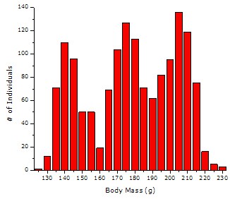
| Measures on a linear scale (e.g., voltage, mass, height, money, etc.) |
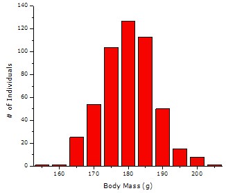 A hypothetical graph of fish weights has the majority of the data centralized and the bars of the graph follow a bell curve. |
Mean. The shape of this data is approximately the same on the left and the right side of the graph, so we call this symmetrical data. For symmetrical data, the mean is the best measurement of central tendency. In this case the mean body mass is 178 grams. |
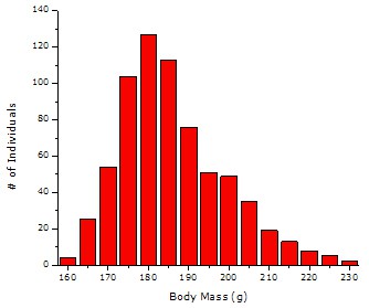 A hypothetical graph of fish weights has the majority of the data in similar groups, but the groups are slightly skewed left of the center of the graph. |
Median. Notice how the data in this graph is non-symmetrical. The peak of the data is not centered, and the body mass values fall off more sharply on the left of the peak than on the right. When the peak is shifted like this to one side or the other, we call it skewed data. For skewed data, the median is the best choice to measure central tendency. The median body mass for this skewed population is 185 grams. | |
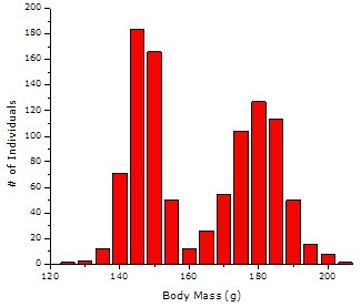 A hypothetical graph measures the weights of male and female fish creating two bell curves on one graph. Each gender of fish has its own central tendency so the separation of data is very noticable. |
Notice how this graph has two peaks. We call data with two prominent peaks bimodal data. In the case of a bimodal distribution, you may have two populations, each with its own separate central tendency. Here one group has a mean body mass of 147 grams and the other has a mean body mass of 178 grams. | |
 A hypothetical graph of a variety of fish has three distinct peaks in the data. Three species of fish have distinct weights but the outlier weights are hard to differentiate. |
None. Notice how this graph has three peaks and lots of overlap between the tails of the peaks. We call this multimodal data. There is no single central tendency. It is easiest to describe data like this by referring to the graph. Don't use a measure of central tendency in this case, it would be misleading. | |
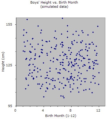 A hypothetical scatterplot showing a boys birth month and height. The plot has data points spread across the entire graph in no discernable pattern. With no pattern visible, we can conclude that a boys birth month and height are not directly correlated. |
None. In this case, the data is scattered all over the place. In some cases, this may indicate that you need to collect more data. In this case there is no central tendency. |
Range, Variance, and Standard Deviation
Measures of Dispersion: Range, Variance, and Standard Deviation
Measures of central tendency describe the "average" of a data set. Another important quality to measure is the "spread" of a data set. For example, these two data sets both have the same mean (5):
data set 2: 1, 2, 4, 5, 7, 11 .
Although both data sets have the same mean, it is obvious that the values in data set 2 are much more scattered than the values in data set 1 (see the following graphs). For which data set would you feel more comfortable using the average description of "5"? It would be nice to have another measure to describe the "spread" of a data set. Such a measure could let us know at a glance whether the values in a data set are generally close to or far from the mean.
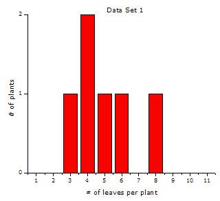
A histogram measures the number of plants that have a certain number of leaves. All plants have different number of leaves ranging from 3 to 8 (except for 2 plants who both have 4 leaves). The difference between the highest number of leaves and lowest number of leaves is 5 so the data has relatively low variance.
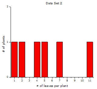
A histogram measures the number of plants that have a certain number of leaves. All plants have different number of leaves ranging from 1 to 11. The difference between the plant with the highest number of leaves and the lowest number of leaves is 10 so the data has relatively high variance.
The descriptive statistics that measure the quality of scatter are called measures of dispersion. When added to the measures of central tendency discussed previously, measures of dispersion give a more complete picture of the data set. We will discuss three such measurements: the range, the variance, and the standard deviation.
Range
The range of a data set is the simplest of the three measures. The range is defined by the smallest and largest data values in the set. The range of data set 1 is 3–8. What is the range of data set 2?
The range gives only minimal information about the spread of the data, by defining the two extremes. It says nothing about how the data are distributed between those two endpoints. Two other related measures of dispersion, the variance and the standard deviation, provide a numerical summary of how much the data are scattered.
For more advanced material, see Variance & Standard Deviation.