Variance & Standard Deviation
It would be useful to have a measure of scatter that has the following properties:
- The measure should be proportional to the scatter of the data (small when the data are clustered together, and large when the data are widely scattered).
- The measure should be independent of the number of values in the data set (otherwise, simply by taking more measurements the value would increase even if the scatter of the measurements was not increasing).
- The measure should be independent of the mean (since now we are only interested in the spread of the data, not its central tendency).
Both the variance and the standard deviation meet these three criteria for normally-distributed (symmetric, "bell-curve") data sets.
The variance (σ2) is a measure of how far each value in the data set is from the mean. Here is how it is defined:
- Subtract the mean from each value in the data. This gives you a measure of the distance of each value from the mean.
- Square each of these distances (so that they are all positive values), and add all of the squares together.
- Divide the sum of the squares by the number of values in the data set.
The standard deviation (σ) is simply the (positive) square root of the variance.
The Summation Operator
In order to write the equation that defines the variance, it is simplest to use the summation operator, Σ. The summation operator is just a shorthand way to write, "Take the sum of a set of numbers." As an example, we'll show how we would use the summation operator to write the equation for calculating the mean value of data set 1. We'll start by assigning each number to variable, X1–X6, like this:
| Data Set 1 | |
|---|---|
| Variable | Value |
| X1 | 3 |
| X2 | 4 |
| X3 | 4 |
| X4 | 5 |
| X5 | 6 |
| X6 | 8 |
Think of the variable (X) as the measured quantity from your experiment—like number of leaves per plant—and think of the subscript as indicating the trial number (1–6). To calculate the average number of leaves per plant, we first have to add up the values from each of the six trials. Using the summation operator, we'd write it like this:

which is equivalent to:

or:

Obviously the sum is a lot more compact to write with the summation operator. Here is the equation for calculating the mean, μx, of our data set using the summation operator:

The general equation for calculating the mean, μ, of a set of numbers, X1 – XN, would be written like this:

Sometimes, for simplicity, the subscripts are left out, as we did on the right, above. Doing away with the subscripts makes the equations less cluttered, but it is still understood that you are adding up all the values of X.
The Equation Defining Variance
Now that you know how the summation operator works, you can understand the equation that defines the population variance (see note at the end of this page about the difference between population variance and sample variance, and which one you should use for your science project):

The variance (σ2), is defined as the sum of the squared distances of each term in the distribution from the mean (μ), divided by the number of terms in the distribution (N).
There's a more efficient way to calculate the standard deviation for a group of numbers, shown in the following equation:

You take the sum of the squares of the terms in the distribution, and divide by the number of terms in the distribution (N). From this, you subtract the square of the mean (μ2). It's a lot less work to calculate the standard deviation this way.
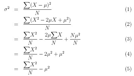
It's easy to prove to yourself that the two equations are equivalent. Start with the definition for the variance (Equation 1, below). Expand the expression for squaring the distance of a term from the mean (Equation 2, below).

Now separate the individual terms of the equation (the summation operator distributes over the terms in parentheses, see Equation 3, above). In the final term, the sum of μ2/N, taken N times, is just Nμ2/N.
Next, we can simplify the second and third terms in Equation 3. In the second term, you can see that ΣX/N is just another way of writing μ, the average of the terms. So the second term simplifies to −2μ2 (compare Equations 3 and 4, above). In the third term, N/N is equal to 1, so the third term simplifies to μ2 (compare Equations 3 and 4, above).
Finally, from Equation 4, you can see that the second and third terms can be combined, giving us the result we were trying to prove in Equation 5.
As an example, let's go back to the two distributions we started our discussion with:
data set 2: 1, 2, 4, 5, 7, 11 .
What are the variance and standard deviation of each data set?
We'll construct a table to calculate the values. You can use a similar table to find the variance and standard deviation for results from your experiments.
| Data Set | N | ΣX | ΣX2 | μ | μ2 | σ2 | σ |
|---|---|---|---|---|---|---|---|
| 1 | 6 | 30 | 166 | 5 | 25 | 2.67 | 1.63 |
| 2 | 6 | 30 | 216 | 5 | 25 | 11.00 | 3.32 |
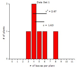
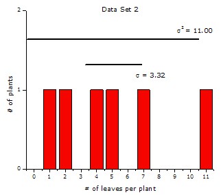
Although both data sets have the same mean (μ = 5), the variance (σ2) of the second data set, 11.00, is a little more than four times the variance of the first data set, 2.67. The standard deviation (σ) is the square root of the variance, so the standard deviation of the second data set, 3.32, is just over two times the standard deviation of the first data set, 1.63.

A histogram showing the number of plants that have a certain number of leaves. All plants have a different number of leaves ranging from 3 to 8 (except for 2 plants that have 4 leaves). The difference between the highest number of leaves and lowest number of leaves is 5 so the data has relative low variance.

A histogram showing the number of plants that have a certain number of leaves. All plants have different number of leaves ranging from 1 to 11. The difference between the plant with the highest number of leaves and the lowest number of leaves is 10, so the data has relatively high variance.
The variance and the standard deviation give us a numerical measure of the scatter of a data set. These measures are useful for making comparisons between data sets that go beyond simple visual impressions.
Population Variance vs. Sample Variance
The equations given above show you how to calculate variance for an entire population. However, when doing science project, you will almost never have access to data for an entire population. For example, you might be able to measure the height of everyone in your classroom, but you cannot measure the height of everyone on Earth. If you are launching a ping-pong ball with a catapult and measuring the distance it travels, in theory you could launch the ball infinitely many times. In either case, your data is only a sample of the entire population. This means you must use a slightly different formula to calculate variance, with an N-1 term in the denominator instead of N:
 Image Credit: Ben Finio, Science Buddies / Science Buddies
This is known as Bessel's correction.


