Linear & Nonlinear Springs Tutorial
Introduction
This tutorial provides a basic summary of linear and nonlinear springs and their associated equations for force, stiffness, and potential energy. You will need a basic understanding of calculus (integrals and derivatives) to understand the section on nonlinear springs.
Definitions
A linear spring is one with a linear relationship between force and displacement, meaning the force and displacement are directly proportional to each other. A graph showing force vs. displacement for a linear spring will always be a straight line, with a constant slope.
A nonlinear spring has a nonlinear relationship between force and displacement. A graph showing force vs. displacement for a nonlinear spring will be more complicated than a straight line, with a changing slope.
Equations at a Glance
| Linear Springs | Nonlinear Springs | |
|---|---|---|
| Force: |
|
|
| Stiffness: |
|
|
| Potential Energy: |
|
|
|
Credits
Author: Ben Finio, Ph.D., Science Buddies
Linear Springs
If you have ever learned about springs in your physics classroom or elsewhere, this symbol might be familiar:
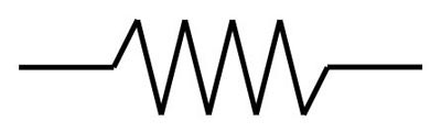 Image Credit: Ben Finio, Science Buddies / Science Buddies
Figure 1. Common symbol for a spring
The symbol in Figure 1 above is designed to look like a typical "coiled" metal spring (see Figure 2). In real life, springs come in all shapes and sizes. However, other objects, like rubber bands, can also act like springs.
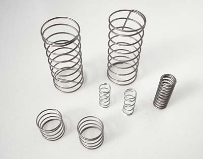 Image Credit: Wikipedia Commons / Public domain
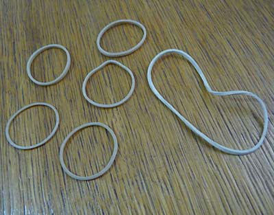 Image Credit: Wikimedia Commons / Creative Commons Attribution-Share Alike 3.0 Unported
Figure 2. Left: several coiled metal springs of different sizes (Wikimedia Commons user Batholith, 2011). Right: Rubber bands , which also come in many shapes and sizes, can also behave like springs — even if they do not resemble the symbol in Figure 1 above (Wikimedia Commons user Chenspec, 2011).
Along with the symbol in Figure 1, you might have seen this equation:
Equation 1:
This equation models the basic physics of a spring — it describes how a spring exerts a force when you push or pull on it. The force (F) (in newtons) is proportional to the displacement (x) (in meters) of the spring - and the force is calculated by multiplying the displacement by the spring constant (k) (in newtons/meter). You may also hear the spring constant referred to as the stiffness of the spring. It is important to note that the x in Equation 1 is not the total length of the spring - it is the difference between the spring's current length and its neutral length or rest length (these terms are interchangeable). So, you might also see Equation 1 written as:
Equation 2:
(where x is the spring's current length and x0 is the spring's neutral length)
or:
Equation 3:
(where Δx is the difference between the spring's current length and its neutral length).
Equations 1, 2, and 3 all mean the same thing — you just need to keep track of how you are defining x.
If we take Equation 1 and use it to plot the force vs. displacement curve for a spring (let us pick k = 100 N/m), we get the graph in Figure 3 below. Note how the force vs. displacement curve is a straight line - so we call this a linear spring. Also note that we can rearrange Equation 1:
Equation 4:
The rearrangement in Equation 4 tells us that k is the slope of the line in Figure 3. So, if you can create a force vs. displacement graph for a spring in one of your experiments (the easiest way to do this is to hang weights from the spring and measure its displacement with a ruler), and the resulting curve appears linear, you can use Equation 4 to calculate the spring constant. If the resulting curve is not a straight line, you will need to go to the Nonlinear Springs tab.
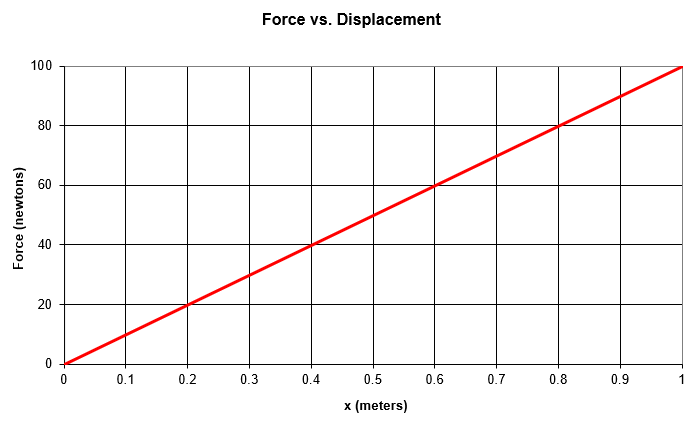 Image Credit: Ben Finio, Science Buddies / Science Buddies
Figure 3. The force vs. displacement graph ( ) for a linear spring with a spring constant of k = 100 N/m.
You may also be familiar with the equation for the potential energy (or PE) stored in a spring:
Equation 5:
where again, depending on the method of expressing the variable x, this could also be written as:
Equation 6:
or:
Equation 7:
But where did this equation come from? We will show you how to arrive at Equation 5 in two ways — with and without calculus.
Without Calculus
For linear springs, you can calculate the potential energy without calculus. To do so, we need another common physics equation:
Equation 8:
This equation says that the work (or W) (in joules) done by a force (or F) is equal to the product of that force and the distance (d) over which it acts. This also means that you can calculate the total work done, and thus the potential energy, by calculating the area under a force-displacement curve - which is exactly what we have in Figure 3! We know that the area under a force-displacement curve for a linear spring will always be a right triangle, and the area of a right triangle is:
Equation 9:
So, for a linear spring, we have:
Equation 10:
and there you have it! This is how you arrive at Equation 5. Figure 4 below helps illustrate how you calculate the area.
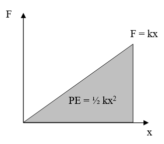 Image Credit: Ben Finio, Science Buddies / Science Buddies
Figure 4. The area under the force-displacement curve for a linear spring forms a right triangle, and the area of that triangle is used to calculate the potential energy stored in the spring.
With Calculus
If you are familiar with calculus, then you probably realize that all we did in the section above was take a special case of an integral - in this case, the area of a triangle. More generally, we want to integrate Equation 8 to arrive at the stored potential energy (this will be useful in the nonlinear springs section). So, the work done by a varying force F(u) over a distance x is:
Equation 11:
where u is a dummy variable we have inserted for distance (remember that it is considered bad mathematical form to use the same variable for both the limits of the integral and inside the integral - this could get you in trouble with your calculus teacher!). If we substitute Equation 1 from above into Equation 11 and replace W with PE (you can do this because, assuming there are no frictional losses, the work required to stretch the spring will be exactly equal to the resulting potential energy stored in the spring), we determine that:
Equation 12:
and again, we have arrived at Equation 5!
Nonlinear Springs
The preceding section deals with linear springs, which follow a simple set of equations and behave "nicely." However, springs might not actually behave like that in real life. For example, Figure 5 shows a force-displacement curve that we measured for a rubber band in the Science Buddies project, Launch Time: The Physics of Catapult Projectile Motion.
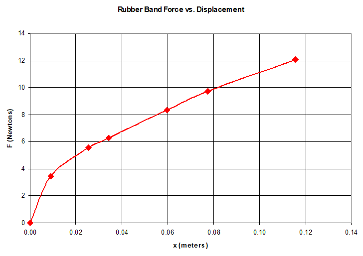 Image Credit: Ben Finio, Science Buddies / Science Buddies
Example graph shows the force needed to stretch a rubber band. The force required increases sharply at first, and then increases less as displacement increases (forming a convex curve).
Figure 5. Measured force vs. displacement curve for a rubber band. This curve is nonlinear, so it does not follow Equation 1.
Do you see a problem? It is not a straight line. This means that the rubber band does not follow Equation 1 (in the Linear Springs section, where F=kx) for force as a function of displacement — and therefore it will not follow Equation 5 (in the Linear Springs section, where PE=1/2 k x²) for potential energy. The rubber band behaves as a nonlinear spring. We can use a curve-fitting tool to find the equation for the line. In this case, the equation for the data in Figure 5 is:
Equation 13:
As in the Linear Springs section, F is force in newtons and x is displacement from the spring's neutral position in meters. The values of 33.55 and 0.4871 are specific to the rubber band from our catapult project, so we can write a more general form of this equation with two constants, a and p, where a is the coefficient and p is the exponent:
Equation 14:
This type of equation is called a power law because the variable x is raised to the power of p. The values of a and p will be different for different rubber bands. However, you cannot always assume that a nonlinear spring will follow a power law! That just happened to be the case in the catapult experiment — there are other potential equations for the force vs. displacement curve, such as exponential, polynomial, or logarithmic. We do not have space to explain these different types of curves here — the point is that you should always perform an experiment to create a force vs. displacement curve for your spring, then find out what type of curve fits the data best.
Now, notice how Equation 14 above is different from Equation 1 in the Linear Springs section. Because we have a nonlinear spring, the slope of the force-displacement curve is not constant. The definition of k as "the slope of the force-displacement curve" is still true, but now that value can change. In general, you can take the derivative of the force-displacement curve at any point to find the stiffness (we do not call it the "spring constant" anymore, because it is not actually a constant):
Equation 15:
For the rubber band in our project, we are going to round the exponent p to ½. We can then plug Equation 13 into Equation 15, and we arrive at our equation for the stiffness of the rubber band:
Equation 16:
Figure 6 shows the stiffness vs. displacement curve for this particular rubber band. Notice how, as the rubber band stretches more, the stiffness decreases instead of remaining constant. This means that the rubber band actually gets weaker as you stretch it.
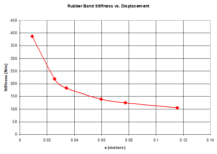 Image Credit: Ben Finio, Science Buddies / Science Buddies
Example graph showing the stiffness of a rubber band as it is stretched apart. The stiffeness decreases sharply at first, and then decreases less as displacement increases forming a concave curve.
Figure 6. Stiffness vs. displacement curve for the rubber band, which behaves as a nonlinear spring. The stiffness decreases with increasing displacement, instead of remaining constant.
We also want to calculate the potential energy of this nonlinear spring. We can use the general equation:
Equation 17:
Remember that PE is potential energy and u is a dummy variable that we use for displacement, because we are already using x for the limit of the integral. In the case of our rubber band, this evaluates to:
Equation 18:
Notice how this turns out quite different from Equation 5 (from the Linear Springs section). Remember that Equation 18 is specific to the rubber band used in this catapult project — for a general nonlinear spring, you will need to use Equation 17 to calculate the potential energy after you have found an equation for F(x).