Abstract
The "impossible arrow" is an amazing optical illusion: an arrow that always seems to point to the right, even when you rotate it 180°. If you place the arrow in front of a mirror, however, its reflection points to the left! How does this illusion work? Can you design your own "impossible" shapes? Try this project and find out!Summary
Based on the work of Dr. Kokichi Sugihara
Thanks to Dr. Mark Veillette for helpful contributions and Python code
/-/https/i.ytimg.com/vi/n--zawliqvA/maxresdefault.jpg)
Objective
Design and 3D print your own seemingly impossible shapes that result in an optical illusion called "anomalous mirror symmetry."
Introduction
The "impossible arrow" is an optical illusion designed by Dr. Kokichi Sugihara. As the video shows, you can place the object so the arrow appears to point to the right. When you rotate the shape 180°, it appears to point to the right again!
Place the arrow in front of a mirror, though, and its reflection appears to point to the left (Figure 1). Dr. Sugihara calls this effect "anomalous mirror symmetry," and you can read about it in his 2016 paper, linked in the Bibliography.
The object looks like an arrow pointing to the right, but its reflection seems to show an arrow pointing to the left.
Figure 1. The "impossible arrow" illusion. The arrow appears to point to the right, but its reflection in the mirror points to the left.
What shape is the object, really? Take a look at Figure 2 and you will see that, when you view it from the top or the side, the shape does not look like an arrow at all.
Figure 2. Top and side views of the "impossible arrow" reveal that it does not look like an arrow at all when viewed from these angles.
This illusion works because, from the correct viewing angle, your brain interprets the top of the object as flat. You can see in the side view in Figure 2, however, that the top and bottom surfaces are not flat at all — they follow a three-dimensional path.
The illusion works from both sides. In other words, you can rotate the object 180° and it will still look like the original shape, an arrow pointing to the right. Alternatively, you can put the object in front of a mirror and its reflection will appear flipped so the arrow points to the left.
This illusion works for other shapes as well. Examples from Dr. Sugihara's paper include a boat, a car, and a fish.
In this project, you will choose your own 2D shape and make it into a 3D shape that produces an "anomalous mirror symmetry" illusion.
The process to generate the three-dimensional shape based on a desired two-dimensional shape is explained in detail in the paper, but we will summarize it here.
Note: Depending on what math classes you have taken in school, you might not have seen all of the vocabulary used here, and that is OK. You can follow the procedure for this project to make your own 3D illusion shapes even if you do not understand the math in this background section.
First, you will create the outline of a two-dimensional shape in the x-y plane. The shape is defined by top and bottom curves, which we will call a1 and a2 (Figure 3). Note: The term "curve" in mathematics refers to a path that does not have be straight, although it can be. In other words, technically, a straight line can still be called a "curve." So we still refer to the paths in Figure 3 as "curves" even though they are made from straight line segments.
Figure 3. A two-dimensional drawing of an arrow in the x-y plane, with top curve a1 and bottom curve a2.
Each curve must be a function of x, meaning it has only one y-value per x-value in the domain.
The two curves must meet at their endpoints on the x-axis, forming a closed curve. For simple shapes, you can just plot some points in the function manually. Functions can also be defined using equations that calculate a y value for each x value in the domain. For example, the equation for a straight line is usually written in slope-intercept form:
Equation 1:
Where m is the slope and b is the y-intercept of the line. If you know that a line goes through two points (x1, y1) and (x2, y2), you can also write the equation in two-point form:
Equation 2:
You can use piecewise functions — a combination of functions, each of which only applies on a certain section of the domain for x. This will allow you to draw shapes made out of multiple line segments. Figure 4 shows the piecewise functions for the arrow in Figure 3. You can use other mathematical functions (such as quadratic, polynomial, or trigonometric functions) to generate more complex shapes.
/-/https/www.sciencebuddies.org/cdn/Files/18527/5/piecewise-functions.png)
The equations for the different segments of the curve, from left to right, are: y=5x+5; y=0.5; y=5x+1; y=-x-1
Figure 4. Piecewise functions that define the top curve a1 of the arrow shape.
Dr. Sugihara's paper contains equations that convert these two-dimensional curves into three-dimensional curves that look like the two-dimensional shape when viewed from an angle θ (Figure 5). The view angle is defined downward from a horizontal line that is parallel to the y-axis, so looking at the shape directly from the side would be a view angle of 0°, and looking at the shape from directly above would be a view angle of 90°.
/-/https/www.sciencebuddies.org/cdn/Files/18528/5/view-angle-definition.png)
A dashed line parallel to the y axis is offset in the positive z direction, with an angle theta defined downward from that line.
Figure 5. Definition of the view angle θ.
The equations to convert the 2D curves a1 and a2 into 3D curves c1 and c2 are:
Equation 3:
Equation 4:
where
Equation 5:
"tan" is short for tangent, a trigonometric function. A 45° viewing angle works well, and tan(45°)=1. If you want to experiment with other viewing angles, you will need to calculate the tangent of the desired angle. (Make sure you know whether your calculator is set to degrees or radians, or use an online calculator that lets you select the units.)
What is the result? You can draw a two-dimensional shape like the arrow in Figure 3 either by plotting the points manually or by using piecewise functions. Then, you plug the y-values for your curves a1 and a2 (whether they are points you plotted manually or calculated using an equation) into equations 3 and 4 to find the x, y, and z coordinates for the three-dimensional curves c1 and c2.
When you plot these curves in 3D space, they look nothing like an arrow unless you view along the y axis, looking down at the angle θ (Figure 6). If you keep the downward view angle θ constant and spin the shape around the z axis, you will see the 2D shape only when your view is aligned with the y axis (Figure 7). Even when the shape is rotated a full 180°, it still looks like the original 2D shape — in this case, an arrow pointed to the right.
/-/https/www.sciencebuddies.org/cdn/Files/18529/6/3D-curve-theta.png)
All three views are aligned along the y axis but at three different downward view angles: 90 degrees, 45 degrees, and 0 degrees. The 2D arrow shape is only visible at the 45-degree view angle.
Figure 6. Three different views of the 3D curves c1 and c2. Top view: Looking directly down at the curves (θ=90°). 3D view: Looking down at the shape at a θ=45° angle. Side view: Looking at the shape directly from the side (θ=0°).
Rotations about the z axis of 0 degrees, 45 degrees, 135 degrees, and 180 degrees. The 2D arrow is only visible in the 0 degree and 180 degree views. In both cases it looks like the arrow is pointing to the right.
Figure 7. Multiple views of the shape with a constant downward view angle θ=45° while rotating the shape around the z-axis. The 2D arrow is only visible when the view is aligned with the y-axis. Regardless of whether the view is oriented with the positive or negative y axis, it looks like the arrow is pointing to the right. If you find it difficult to visualize this rotation, remember to watch the video at the beginning of the project.
While this 3D curve works to generate the illusion on a computer screen, it does not work for 3D printing. The curve has zero thickness. If you want to 3D print something, you need a model of a solid object. To do that, you will need to generate an STL file. An STL is a file originally designed for a type of 3D printing called stereolithography. While the acronym may vary depending on where you look, STL stands for either standard triangle language or standard tessellation language. An STL represents a solid object using triangles to define its surface. An STL file of a cube, for example, will consist of twelve triangles, two on each of the six faces of the cube (Figure 8).
/-/https/www.sciencebuddies.org/cdn/Files/18531/5/cubes-STL.png)
Figure 8. Left: A cube plotted in 3D space. Right: An STL representation of the same cube, with each face broken up into two triangles.
To generate a solid 3D shape, first we will make a copy of our curve and shift it upward in the z direction by a distance equal to the desired thickness of our shape (Figure 9). This creates the top and bottom edges of the 3D shape.
/-/https/www.sciencebuddies.org/cdn/Files/18532/5/3D-curves-offset.png)
Figure 9. 3D curves offset in the z direction to create the top and bottom edges of the 3D shape.
Next, we need to fill in the surface of the shape with triangles. This process would be difficult to do by hand, but luckily a computer program can do it for you (Figure 10). The end result is a 3D shape format that can be exported for viewing in a computer-aided design (CAD) program (Figure 11) or for 3D printing.
Figure 10. 3D shape with the surface filled in with triangles.
Figure 11. The STL file imported into a CAD program (Tinkercad). Note that some of the edges visible in Figure 8 are not visible in the CAD program. If the triangles are in the same plane, the CAD program does not draw their edges.
In this project, you will use either MATLAB or Python code that automatically generates the 3D shape and exports an STL file based on the original 2D shape. Defining the original 2D shape is up to you! You can plot the points in the shape manually or define it using functions. Then, you can choose whether you just want to view the illusion on a computer screen, open it in a CAD program, or 3D print it.
What types of illusions can you generate? Do certain shapes not work with the illusion? Try it and find out!
Technical Note: Parametric Curves
Technically, Dr. Sugihara's paper defines the top and bottom curves a1 and a2 as parametric curves, meaning their x, y, and z coordinates are defined as functions of the parameter t:
Equation 6:
Equation 7:
Both curves must be monotone in x, meaning each x value can only occur once on the curve.
This means that the curves c1 and c2 are also parametric and defined as functions of t, not x:
Equation 8:
Equation 9:
These are the equations you will see if you read Dr. Sugihara's paper. Since many students will not have learned parametric functions, Science Buddies has simplified the equations in this project to just be functions of x.
Terms and Concepts
- Optical illusion
- Curve
- Function
- Domain
- Closed curve
- Slope-intercept form
- Slope
- Y-intercept
- Two-point form
- Piecewise
- Tangent
- Radians
- STL
- Stereolithograpy
- Standard triangle language
- Standard tessellation language
- Parametric curve
- Monotone
- Computer-aided design (CAD)
Questions
- How does the "anomalous mirror symmetry" illusion work?
- How do you generate a solid shape from a zero-thickness 3D curve?
- How does an STL file represent a 3D object?
Bibliography
- Sugihara, K. (2016). Anomalous Mirror Symmetry Generated by Optical Illusion. Symmetry. Retrieved May 4, 2022.
- Prisco, J. (2018, May 15). Master of illusion: Kokichi Sugihara's 'impossible' objects. CNN. Retrieved May 4, 2022.
- Math is Fun (n.d.). What is a Function?. Retrieved May 10, 2022.
- Math is Fun (n.d.). Domain of a Function. Retrieved May 10, 2022.
- Math is Fun (n.d.). Piecewise Functions. Retrieved May 10, 2022.
- All3DP (2021, Oct 28). The STL File Format Simply Explained. Retrieved May 4, 2022.
- Google (n.d.). Welcome to Colab. Retrieved May 9, 2022.
- MathWorks, Inc. (n.d.). Getting Started with MATLAB. Retrieved May 9, 2022.
Materials and Equipment
- Computer with one of these two programming options:
- MATLAB. Check whether you have access to MATLAB through your school. If not, you can purchase your own student version or use a 30-day free trial.
- Google Colab, a programming environment that lets you run Python code in your web browser. Colab is free and you do not need to download anything.
- Access to a 3D printer
- If you do not have your own printer, check if you have access to one at your school, a local library, or a makerspace.
- You can also use an online 3D printing service like Shapeways, i.Materialise, or Sculpteo. Note: It may take more than a week for your parts to arrive if you use an online service.
- Spreadsheet program like Microsoft Excel® or Google Sheets®
- Optional: Graph paper (useful for sketching shapes by hand)
- Optional: Mirror
- Lab notebook
Experimental Procedure
- Make sure you understand the requirements for your 2D shape. (If you have not already done so, go back and read the Background section for this project).
- Your shape should consist of upper and lower curves a1 and a2.
- Each curve should be a function of x (each curve has only one y-value per x-value).
- Each curve should start at the point (-1,0) and end at the point (1,0) on the x-axis, forming a closed curve.
- The curves do not have to be symmetric about the x-axis, even though they are symmetric in the example arrow shape.
- Design your 2D shape. There are two different ways you can do this:
- Draw your shape by hand on graph paper. Label the (x,y) coordinates of each point in increments of 0.1 along the x-axis (Figure 12). You can enter these points directly in MATLAB or Python later in the procedure. This approach works well for simple shapes.
- Design your shape in a spreadsheet program like Microsoft Excel or Google Sheets (Figure 13). You can do this by defining piecewise functions of x, entering the equations in your spreadsheet, graphing them, and then changing the functions to see how they affect the shape.
This approach works well for more complex shapes, making it easier to define more points (for example, in increments of 0.01 on the x axis instead of 0.1) or to use equations to define more complex curves. You will need to export your spreadsheet as a CSV file with three columns: the x-coordinate, the y-coordinate of a1, and the y-coordinate of a2. Make sure each column includes a header, with the data starting in the second row. An example xlsx file and an example csv file are available for download.
Figure 12. A 2D drawing of an arrow in the x-y plane with points drawn in increments of 0.1 along the x-axis. Some of the points have their (x,y) coordinates labeled as examples.
The y coordinates are defined by equations. On the right is a graph of the resulting arrow.
Figure 13. The same arrow from Figure 12 designed in Microsoft Excel, with more points (increments of 0.05 on the x-axis) and with the y-coordinates defined by equations instead of being entered manually.
- Depending on which programming language you want to use, follow one of these two steps:
- For MATLAB, download impossible_shape_generator.m, save it on your computer, and open it in the MATLAB editor. You can also download CSV files for the boat, fish, and car shapes from Dr. Sugihara's paper.
- For Python, make a copy of this Google Colab notebook to your personal Google Drive by clicking the "Copy to Drive" button at the top of the screen. Google Colab is an environment that lets you run Python code directly in a web browser. You do not need to download anything.
- Each program comes loaded with a default arrow shape. Do not change anything yet — just run the program to see how it works. Run the code one section at a time, either using the Run and Advance button in the Section part of the MATLAB menu or the Run Cell button (that looks like a Play button) in the top left of each section in Google Colab. Read the on-screen instructions for each section.
Each program will generate six figures (Figure 14). It is easier to understand the figures if you run the code in sections and look at them one at a time, instead of running the whole program at once.
- Figure 1: Plot of the original 2D shape in the x-y plane.
- Figure 2: 3D plot of the curves c1 and c2.
- Figure 3: 3D plot of the original curves c1 and c2, and additional curves offset in the z direction, forming the edges of a 3D shape.
- Figure 4: 3D plot of all the vertices on the top and bottom edges of the 3D shape. These vertices will be connected with triangles to form the STL file.
- Figure 5: 3D plot of the surface triangles using "method 1." This method adds vertical triangles to form the side walls of the shape, then adds triangles connecting the opposite edges to form the top and bottom surfaces of the shape.
- Figure 6: 3D plot of the surface triangles using "method 2." This method adds vertical triangles to form the side walls (the same as method 1), but it connects triangles to a central point to form the top and bottom surfaces of the shape.
The code will also save two STL files, one for each method of adding triangles to the top and bottom surfaces of the shape. For MATLAB, these files will be saved in the same directory as your MATLAB program. For Python, your browser will prompt you to download and save the files.
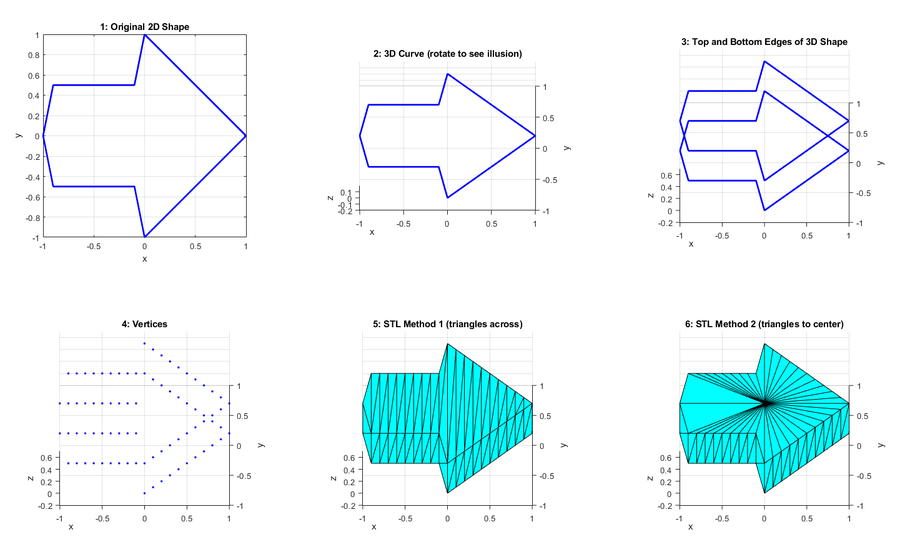
Figure 14. Example output of Figures 1–6 from the MATLAB program. - For each of the 3D graphs, try rotating the graph so you can see the effect of the illusion. The graphs should load with the correct default view so you see the illusion (like the 2D arrow in Figure 14).
- Look at the graph from the top or the side. Does it look anything like the original 2D shape?
- "Spin" the shape about the z axis. In other words, imagine that you have the shape sitting flat on the table in front of you. Spin it while keeping it flat on the table (do not flip it over). What do you see when you rotate the shape a full 180°?
- Now, try entering your own 2D shape in the program. Read the comments in the program you are using to learn how to do this. You will have the option to type the (x,y) coordinates of the points directly into the program manually, or to load them from a CSV file.
- Re-run the program with your new 2D shape and look at each of the resulting figures. Try rotating the plots to different angles again to view the illusion. Note: The MATLAB program will automatically change the names of the output STL files each time you run it, so you do not need to worry about accidentally overwriting previous files.
- Depending on how well the illusion works with the solid 3D shapes, you may want to change the design of your 2D shape. You can also change the height and viewing_angle variables in the code to change the height of the 3D shape and the view angle at which the illusion will appear, respectively. Try changing your shape and re-running the code. Note: If you are storing your 2D shapes in CSV files, you should give each iteration a new filename instead of overwriting the same file when you make changes.
- Keep iterating until you are happy with how your illusion appears on a computer screen. Make sure you keep track of your shape iterations in your lab notebook (if you are entering points manually) or in your CSV filenames (if you are using a spreadsheet program).
- Now you are ready to work with your STL file for viewing in a CAD program or for 3D printing. STL files do not include units, so when uploading to a CAD program or 3D printing service you will need to select the units for the shape. You are usually given options in millimeters or inches. Since your shape goes from -1 to +1 on the x axis, inches are a better choice, or your shape will be too small to print.
- Optionally, you can open your STL files in a CAD program. Tinkercad is a good free option for a beginner-friendly CAD program.
- 3D print one or both versions of your shape. Instructions for doing this will vary depending on your printer. If you are using an online 3D printing service (see materials section), follow the instructions on their site to upload your model, select a material, and order your part. In addition to selecting units when you first upload the model, you may also want to scale the model to make it bigger or smaller. Most 3D printer software and online 3D printing services will give you an option to do this.
- Look at your 3D printed shapes.
- What do you see if you look at the shape from directly above or from the side?
- What do you see if you look at the shape from above at roughly a 45° angle or at your chosen viewing angle?
- What happens if you rotate the shape 180° (put the shape flat on the table and spin it)?
- What happens if you put the shape in front of a mirror?
- Are there any differences between the physical 3D printed shape and what you saw on a computer screen?
- Continue to explore your illusion and try improving your shape or designing new ones.
- Can you design a 2D shape that does not work or that "breaks" the illusion?
- Which STL method for the top and bottom triangles works better for the illusion? Is this the same for all shapes?
- Does increasing the resolution (number of points along the x axis) improve the illusion for one or both methods?
/-/https/www.sciencebuddies.org/cdn/Files/18537/6/matlab-output-figure-illusion.png)
Ask an Expert
Global Goals
The United Nations Sustainable Development Goals (UNSDGs) are a blueprint to achieve a better and more sustainable future for all.
/-/https/www.sciencebuddies.org/cdn/Files/19752/5/E-WEB-Goal-09.png)
Variations
- Can you write your own program to do this project in a language other than MATLAB or Python?
- Read one of Dr. Sugihara's other papers, for example, Topology-disturbing objects: a new class of 3D optical illusion. Can you generate your own shapes that result in this type of optical illusion?
Careers
If you like this project, you might enjoy exploring these related careers:
/-/https/careerdiscovery.sciencebuddies.org/cdn/Files/1442/17/unsplash-TXxiFuQLBKQ.jpg)
/-/https/careerdiscovery.sciencebuddies.org/cdn/Files/1011/20/pexels-photo-7375.jpg)

/-/https/img.youtube.com/vi/UYWBtg_DCb4/0.jpg)
/-/https/img.youtube.com/vi/q8udWLU2HQk/0.jpg)
/-/https/img.youtube.com/vi/QUNM-QyM5PA/0.jpg)